You will need a calculator to complete these problems. You may wish to have Windows calculator and Netscape open at the same time so you can switch back and forth between the two of them. To use Windows calculator, click on Start on the Taskbar, then Run. Type calc into the blank, then press the Enter key or click on the OK button. To copy a number from the calculator, press [Ctrl]-C. Then, return to Netscape, click in the desired space, and press [Ctrl]-V to paste the number into that space. Note that, depending on how you round your answers, they may or may not exactly match with what the computer is expecting. Thus, if you click the Did I Get It? buttons, what will be reported is whether or not your answers exactly matched the computers answers. If there is not an exact match, you will need to judge whether your answers are different due merely to rounding discrepancies or to a real error in your calculations.
Two groups of Freshman Biology Lecture students achieved the
following scores on the third test:
Two means and ranges might be close together, causing one to assume the two samples were similar. However, in one sample, the scores could be more closely grouped with only a few at the extremes, and in another sample, the scores could be more widely spread. Thus, it is useful to calculate the variance, and from that, the standard deviation as indicators of how spread out or clustered the data are (dispersion). If you are interested in the variance of only those individuals in your sample, s2 = Σ (Xi X2/n for this finite group of data. However, if this group is a representative sampling of a larger population, then it has been found that (statisticians use σ here rather than s) σ2 = Σ (Xi X2/(n-1) is a better estimate of the population variance. Thus, for our two groups of students:
In a normal distribution, a graph of scores on the x-axis versus number of people who got that score on the y-axis should give a bell-shaped curve with the mean in the center. 68% of the people should be within one standard deviation unit to either side of the mean and 95% should be within two units of the mean.
Luckily, most scientific calculators as well as the PC in the bio lab will perform these calculations from entered data and a few simple commands.
When comparing data like these, we could make one of several
hypotheses. Either we could say that there is no difference between the two
groups (the null hypothesis Ho) or that there
is a significant difference of some sort. For plants on two given sites A
and B, hypothesis 1 (H1) might be that density on site A is
greater than on site B, while hypothesis 2 (H2) might be that
density on site B is greater than A. Comparing the means and variances alone
can be misleading, so we must do further statistical testing to determine
whether we can say (with, usually, a 95% confidence level) that, for the null
hypothesis, there is no difference between these two samples or for
H1 and H2 combined, that there is a difference between
them. The test used for this is called the t-test:

Thus, for our two groups of students:
This value is compared to a table of t-scores for a number of possible degrees of freedom [DF]. For one sample, DF = n 1, so for two samples, DF = n1 + n2 - 2 (in this case, Since we want to be 95% certain (0.95) we must look at the t-value for 1.00 0.95 = 0.05. As an alternative hypothesis, let us say there is a difference between the two groups either #1 is higher or lower than #2. Since we have two choices, we need to look at the value of t for 0.05 for the two-tailed test, which is degrees of freedom. Our calculated value might be positive or negative, depending on if we compared #1 to #2 or #2 to #1, so if the absolute value of t is greater than or equal to the table value, we can accept the alternative hypothesis, and if it is less than the table value, we can reject the alternative and accept the null hypothesis. For our two groups of students, our observed value of a difference between our two groups.
A group of ecology students was studying and comparing two
different forest areas by taking 20 sample plots in each area. In each woods
the combined number of sugar plus red maple trees in each of the 20 plots was
found to be:
Calculate the range, mean, s, and σ for the number of maples per plot for each of these two areas. Use a t-test to tell if the number of maples per plot for the two areas is significantly different.
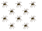
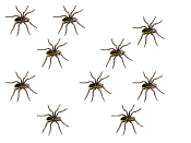
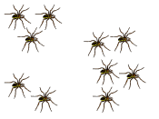
The density of a species is the number of organisms of that species per unit area/volume. The dispersion of a species refers to the spatial distribution of the individuals. Generally, these are arranged in one of three ways: In uniform dispersion, individuals are evenly scattered throughout the habitat. In random dispersion, individuals are scattered throughout the habitat, at random. In clumped dispersion, individuals are clustered together in some locations, while other locations have few/none.
 |
 |
 |
| Figure 1. Uniform | Figure 2. Random | Figure 3. Clumped |
Statistically, it is possible to analyze whether a species is randomly or uniformly dispersed or clumped. Consider the following example:
| plot # | # of ladybugs |
plot # | # of ladybugs |
plot # | # of ladybugs |
|---|
From these data, the following table can be constructed:
For each X (# individ./plot) something called the poisson relative frequency can be calculated by the following formula: prf = (em)(mX/X!). In this equation, e is the base of natural logarithms We can then calculate the following values:
By multiplying the total number of plots (n) by the prf, we can predict how many plots we should expect to have each of the X number of ladybugs out of the total plots, so for
This means that if the species is randomly distributed, most of the plots should have about the same average number of individuals with only a few plots having extremely high or low numbers like a bell-shaped curve. We can, then, compare the observed (O) and expected (E) values to see how closely the observed data fit the expected data is the species really randomly distributed? This can be done by means of a statistical analysis called the chi-square (χ2) test where:
χ2 = Σ[(O E)2/E].
Thus, we can add two more columns to our chart as follows:
This number is then compared to a table of χ2 values. Because we have six different choices for X, degrees of freedom (DF) = 6 1 = 5. Once again, we want to test the data at the 95% level, so we need to look up the value for 0.05. The value corresponding to 0.05 and 5 DF is 11.070. Since χ2calc of the null hypothesis that dispersion is random for this group of individuals (that there is no difference between observed and expected values). Thus, the χ2 test an alternate hypothesis that there is a difference between O and E. If the alternative hypothesis is supported, it is then necessary to figure out whether the organisms are clumped or uniformly distributed. In order to figure out whether the organisms are uniformly dispersed or clumped, a few more calculations must be done to compare the variance (s2) and the mean (m). Another formula for s2 which is easier to use here is: s2 = [ΣX2×O n(m)2]/DF, where (in this example)
For any samples, if m < s2 (or
s2 > m), then the distribution is clumped and if
m > s2, then the distribution is uniform. In this case,
| Degrees of Freedom |
χ2 Value | Critical Values of t | |
|---|---|---|---|
| at P = 0.05 level | one-tailed @ 0.05 | two-tailed @ 0.05 | |
| 1 | 3.841 | 6.314 | 12.706 |
| 2 | 5.991 | 2.920 | 4.303 |
| 3 | 7.815 | 2.353 | 3.182 |
| 4 | 9.488 | 2.132 | 2.776 |
| 5 | 11.070 | 2.015 | 2.571 |
| 6 | 12.592 | 1.943 | 2.447 |
| 7 | 14.067 | 1.895 | 2.365 |
| 8 | 15.507 | 1.860 | 2.306 |
| 9 | 16.919 | 1.833 | 2.262 |
| 10 | 18.307 | 1.812 | 2.228 |
| 11 | 19.675 | 1.796 | 2.201 |
| 12 | 21.026 | 1.782 | 2.179 |
| 13 | 22.362 | 1.771 | 2.160 |
| 14 | 23.685 | 1.761 | 2.145 |
| 15 | 24.996 | 1.753 | 2.131 |
| 16 | 26.296 | 1.746 | 2.120 |
| 17 | 27.587 | 1.740 | 2.110 |
| 18 | 28.869 | 1.734 | 2.101 |
| 19 | 30.144 | 1.729 | 2.093 |
| 20 | 31.410 | 1.725 | 2.086 |
| 21 | 32.671 | 1.721 | 2.080 |
| 22 | 33.924 | 1.717 | 2.074 |
| 23 | 35.172 | 1.714 | 2.069 |
| 24 | 36.415 | 1.711 | 2.064 |
| 25 | 37.652 | 1.708 | 2.060 |
| 26 | 38.885 | 1.706 | 2.056 |
| 27 | 40.113 | 1.703 | 2.052 |
| 28 | 41.337 | 1.701 | 2.048 |
| 29 | 42.557 | 1.699 | 2.045 |
| 30 | 43.773 | 1.697 | 2.042 |
| 31 | 1.696 | 2.040 | |
| 32 | 1.694 | 2.037 | |
| 33 | 1.692 | 2.035 | |
| 34 | 1.691 | 2.032 | |
| 35 | 1.690 | 2.030 | |
| 36 | 1.688 | 2.028 | |
| 37 | 1.687 | 2.026 | |
| 38 | 1.686 | 2.024 | |
| 39 | 1.685 | 2.023 | |
| 40 | 1.684 | 2.021 | |
| 60 | 1.671 | 2.000 | |